To prevent cells from being edited, you can lock them in Google Sheets. This is especially convenient if you’re working on a spreadsheet with others. You may have formulas or functions that you want to make sure no one can change.
What’s nice about the ability to lock cells in Google Sheets is that you have flexibility. You can lock a single cell, a range, column, row, or the entire sheet. In addition, you can choose the permissions for the locked cells. This lets you allow certain people the ability to change them.
Here’s how to lock cells in Google Sheets, adjust the permissions, and unlock the cells for editing later.
Lock specific cells in Google Sheets
Visit Google Sheets, log in, and open the spreadsheet you want to lock cells in. Note: You can also open the spreadsheet from your Google Drive.
Step 1: Select the cells you want to lock. Again, this can be an individual cell, cell range, row, or column.
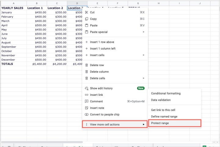
Step 2: Click Data > Protect sheets and ranges from the menu or right-click the selection, move to View more cell actions, and pick Protect range in the pop-out menu.

Step 3: You’ll then see the Protected Sheets and Ranges sidebar open. Confirm that the Range tab is selected. Your chosen cells appear in the range box that you can edit if needed.
Step 4: Optionally, add a description in the Enter a description box.
Step 5: Click Set permissions.

Step 6: When the Range Editing Permissions box appears, you’ll decide who can edit the locked cells or provide a warning if someone tries to edit them.
Option 1: To only display a warning, mark the first option for Show a warning when editing this range.
Option 2: To restrict the editing to certain users, mark the second option for Restrict who can edit this range. Click the drop-down box and pick Only you, Custom, or Copy permissions from another range.
If you select the Custom option, you’ll see a list of those you’re sharing the sheet with at the bottom. Check the boxes to the right of those you want to allow editing permissions. Optionally, you can add more editors at the bottom.

Step 7: Click Done when you finish.
Lock a sheet in Google Sheets
If you want to lock the cells in an entire sheet or want to lock all but certain cells in a sheet, this is also an option.
Step 1: Select any cell and go to Data > Protect sheets and ranges in the menu or right-click the sheet, move to View more cell actions, and pick Protect range.

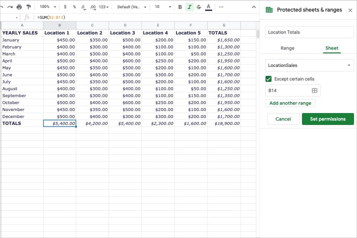
Step 2: When the Protected Sheets and Ranges sidebar opens, click the Sheet tab.
Step 3: Pick the name of the sheet you want to lock from the drop-down list.
Step 4: If you want to lock all but specific cells, check the box for Except certain cells. Add the cell, range, column, or row in the corresponding box. To include more, click Add another range and do the same.
Step 5: Optionally add a description in the Enter a description box.
Step 6: Click Set permissions.

Step 7: When the Range Editing Permissions box appears, choose Option 1 or Option 2 as described above and complete the details.

Step 8: Click Done.
Change permissions for locked cells
There may come a time when you want to adjust the permissions you set for locked cells. You may want to add another editor or remove one.
Step 1: Go to Data > Protect sheets and ranges in the menu or right-click, move to View more cell actions, and pick Protect range.
Step 2: In the Protected Sheets and Ranges sidebar, you’ll see a list of cells or the sheet you’ve locked. Select the one you want to edit.

Step 3: Click Change permissions.

Step 4: Make your changes in the pop-up window and click Done when you finish.
Unlock cells in Google Sheets
If you want to remove the lock you’ve placed on cells or on a sheet, you can do this easily.
Step 1: Go to Data > Protect sheets and ranges in the menu or right-click, move to View more cell actions, and pick Protect range.
Step 2: In the Protected Sheets and Ranges sidebar, you’ll see a list of cells or the sheet you’ve locked. Select the one you want to unlock.

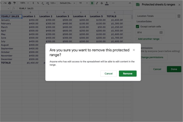
Step 3: Click the trash can icon to the right of the description.

Step 4: Confirm that you want to remove the protection by clicking Remove in the pop-up window.

Protecting data and formulas by locking cells in Google Sheets only takes a few minutes and is worth the time to keep your data safe.
For more, take a look at how to make a graph in Google Sheets for a visual display of your data.


