How to highlight duplicates in Google Sheets

A MacBook owner using Google Sheets.
Image used with permission by copyright holder

If you’ve added the same data more than once by mistake on your spreadsheet or you’re simply looking to find multiple cells that contain the same word, number, or formula, Google Sheets has a simple way to highlight them.

Let’s take a look at how to highlight duplicates in Google Sheets.

Recommended Videos

Difficulty

Easy

Duration

5 minutes

What You Need

  • A computer, laptop, tablet, or phone with access to Google Sheets

Using the Conditional formatting tool

Step 1: Click the cells that you want to include within the search for duplicates. You can choose a column, specific cells, and rows. For demonstration purposes, I have highlighted the A column.

Selecting a column in Google Sheets in order to use it to highlight duplicate data.
Image used with permission by copyright holder

Step 2: Click the Format tab and then select Conditional formatting.

The Conditional formatting tab in Google Sheets.
Image used with permission by copyright holder

Step 3: Within the Conditional format rules section, the Apply to range field will already be filled via the column you’ve selected. In my case, that’s column A. You can change it yourself as well via this field manually.
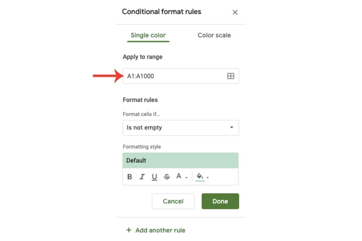
The Apply to range box in Google Sheets for highlighting duplicate data.
Image used with permission by copyright holder

Step 4: Click the Format cells if menu and select Custom formula.

The Format cells if drop-down menu in Google Sheets and the Custom formula is option within that menu.
Image used with permission by copyright holder

Step 5: Within the Value or formula box, enter =countif(A:A,A1)>1. If you’ve not selected the column, but have instead selected the cells starting from, say, either A1 or A2, then the aforementioned formula should still be used.

Entering a custom formula that will highlight duplicate data in Google Sheets’ Custom formula is box.
Image used with permission by copyright holder

Step 6: Click Done. The duplicates will be highlighted in the A column.

Google Sheets also provides further customization options for highlighting duplicates such as making them bold or changing their color.

The Formatting style section for customizing the appearance of how highlighted duplicate data appears.
Image used with permission by copyright holder

Step 7: If you don’t want to see the duplicates highlighted anymore, click the Remove rule button via the trash icon.

The trash icon button for removing highlighted duplicate data in Google Sheets.
Image used with permission by copyright holder

Deleting duplicates in Google Sheets

If you find any duplicates within your spreadsheet, it may be a part of your data and thus doesn’t need to be deleted. But in case you do need to remove it, Google allows you to perform this function with the Remove duplicates tool.

Step 1: Click the column where it contains duplicates. I’ve clicked column A.

Step 2: Click the Data tab > Data cleanup > Remove duplicates.

The Remove duplicates tool in Google Sheets.
Image used with permission by copyright holder

Step 3: Select the Remove duplicates button. If you’ve applied the highlight duplicates formula for other columns such as column B and want to remove them as well, then click the Expand to A:B option and then select the Remove duplicates button.

The Remove duplicates button in Google Sheets.
Image used with permission by copyright holder

If you're a new Google Sheets user, we have more helpful tips and tricks in our guides on how to search and how to merge cells in Google Sheets.

Zak Islam
Former Digital Trends Contributor
Zak Islam was a freelance writer at Digital Trends covering the latest news in the technology world, particularly the…
How to wrap text in Microsoft Excel
Stock photo of man using laptop

Microsoft Excel may be a productivity app that emphasizes numbers, but it has useful tools for text as well. For instance, that handy spreadsheet app will let you wrap text. And getting it done is a breeze. In this guide, we'll show you two ways to wrap text using Microsoft Excel: Manually and automatically.

Read more
How to multiply in Excel
Stock photo of woman using laptop at desk

While it's not as easy as tapping a few keys on a calculator, you can use Microsoft Excel to perform simple math, such as multiplying numbers. In order to do this, you'll need to learn Excel's language a bit. But don't worry, in this guide, we'll go over what you need to know as we show you how to multiply in Excel.

We'll review four different ways to multiply in Excel: Simple multiplication within a cell, multiplying numbers from different cells, multiplying ranges of numbers, and multiplying each number of a column by a constant.

Read more
How to freeze rows and columns in Excel
Microsoft Excel opened on a desktop computer.

If you’ve ever worked with an enormous Excel spreadsheet, you’ll know just how daunting all those rows and columns can be. Once you’re over 10 or 15 different values and labels, it can get pretty difficult to hang onto any info you’ve gleaned from these early cells. Fortunately, there’s a simple way to lock those little rectangular boxes of information.

The name of the game is “freezing,” and the execution is about as surface-level as the word. You use Microsoft Excel's built-in function to freeze specific rows and columns (often row or column headers), so when you’re scrolling through, these cells remain stationary on the page.

Read more